Intro

In July 2026 Anthropic’s interpretability team released the paper “Verbalizable Representations Form a Global Workspace in Language Models”. Its main result: inside Claude, among tens of thousands of features for the internal representations of words, they found a subsystem that closely resembles a global workspace from the neuroscientific theory of consciousness.

There’s no public code, but right now the ideas and conclusions are what matter — all of it can be double-checked by hand in a few hours with AI agents. I have a MacBook Pro on M3 Max, 64 GB unified memory. Not an A100 or an H200, but fp32 models up to 7B are easy to push through dozens of backward passes — just slower. The result is JLens: a from-scratch reimplementation, two model families in two sizes each — Qwen2.5-1.5B and Qwen2.5-7B, Gemma-2-2b and Gemma-2-9b — plus a separate battery of checks so as not to pass off self-deception as reproduction.

JLens in two formulas

A token $t$‘s representation at layer $\ell$ is a vector $h_{\ell, t} \in \mathbb{R}^d$. At the end, the transformer normalizes the last residual and multiplies by the unembedding matrix:

$\mathrm{logits}\,=\,W_U\,\cdot\,\operatorname{norm}(h_L)$

A softmax over the logits then gives the next-token probabilities during generation.

• Logit lens (Nostalgebraist, 2020): take an intermediate state $h_\ell$ and interpret it as if it were already final: $\operatorname{softmax}(W_U \cdot \operatorname{norm}(h_\ell))$. It works decently in the upper layers, but turns to noise in the middle of the network: there $h_\ell$ simply lives in a different basis than the one $W_U$ expects.

• JLens — Anthropic’s generalization. We pass the same vector $h_\ell$ through a corpus-averaged linearization of the entire remaining network:

$$\begin{aligned} J_\ell &= \mathbb{E}_{\text{corpus},\; t' \ge t}\!\left[\frac{\partial h_{L,t'}}{\partial h_{\ell,t}}\right] \quad\text{(one } d \times d \text{ matrix per layer)} \\[4pt] \operatorname{lens}_\ell(h) &= \operatorname{softmax}\!\big(W_U \cdot \operatorname{norm}(J_\ell\, h)\big) \\[4pt] v_y &= (W_U J_\ell)_y \quad\text{--- J-vector of token } y \end{aligned}$$

That is, the rows of the matrix $W_U J_\ell$ are the J-vectors of every token in the model’s vocabulary.

If $J_\ell = I$, we recover the ordinary logit lens. Having the J-vectors gives three operations right away:

• steering: $h \leftarrow h + \alpha v_y$, nudge the state toward token $y$
• patching: replace coordinates in the J-vector basis, e.g. «France» with «China»
• ablation: subtract the projection onto the active J-vectors and see what breaks

Computing the Jacobian without a GPU budget

The brute-force way — $d$ backward passes per layer, explicitly building the $d \times d$ matrix. Too expensive, of course, so the paper uses a trick. Into each layer we add a constant zero vector $\delta_l = (0, \dots, 0)$, broadcast across all input positions $t = 1\dots \mathrm{ctx}$

$h_{l,t}' = h_{l,t} + \delta_l,$

and then

$$h_L = f(h_l + \delta_l) \rightarrow \frac{\partial h_L}{\partial \delta_l} = \sum\limits_t \frac{\partial h_L}{\partial h_{l,t}'} \frac{\partial h_{l,t}'}{\partial \delta_l}$$

So $\frac{\partial h_L}{\partial \delta_l} = \sum\limits_t \frac{\partial h_L}{\partial h_{l,t}}$, and this broadcast automatically sums the Jacobians over all input positions $t$.

But that’s not all! Now let’s introduce the right loss function

$G_i = \sum\limits_{t'} h_{L,t',i}$

— the sum of the $i$-th coordinate of the final residual over all positions. A single backward pass from $G_i$ gives row $i$ of the summed Jacobian, and for all layers at once, because all the $\delta_\ell$ hang in one graph. So the whole matrix $J_\ell$ is computed in $d$ passes.

Don’t forget to zero the gradients of $\delta_l$ between the $d$ passes, or PyTorch will accumulate them.

Moreover, for a specific token $y$ we can compute the corresponding row of the Jacobian in a single backward pass. For $k$ target tokens that’s $k$ passes, regardless of the dimension $d$. That’s how the France→China patching and the trial runs work even on 7B — in minutes, not overnight.

Setup and validation

MacBook Pro, Apple M3 Max, 64 GB unified memory, macOS, arm64. PyTorch 2.5.1 on MPS, transformers 5.13.0, everything in fp32 with attn_implementation="eager": finite differences and an averaged Jacobian make no sense without fp32, and eager sidesteps the known MPS problems with softmax attention and NaNs in Gemma-2’s softcap attention.

I took models from two different families: Qwen2.5-1.5B, Qwen2.5-7B and Gemma-2-2b, Gemma-2-9b. Gemma-2 has its own normalization, logit softcap, and embedding scaling. If the method honestly works there too, then it isn’t about the architectural quirks of a single family.

Before trusting any result — four checks. Three are bit-exact: logit_lens(raw h_L) matches the model’s logits to within 0.0, including the whole Gemma zoo of quirks; j_lens(h, I) matches logit_lens(h) to within 0.0; the diagonal of $J$ at the last layer equals exactly $2/(S+1) = \frac{S}{S(S+1)/2}$, where $S = ctx$. The fourth check is finite-difference — $J_\ell \cdot v$ against the directional derivative — and converges with a relative error of 0.85–2.1%. This also rules out the known MPS bug that silently zeros out the Jacobian.

Experiments

1. The Eiffel Tower: JLens sees Paris before the logit lens

Prompt: «The capital of the country where the Eiffel Tower is located is the city of». The correct answer is Paris. We look at the rank of that token across the whole vocabulary, layer by layer.

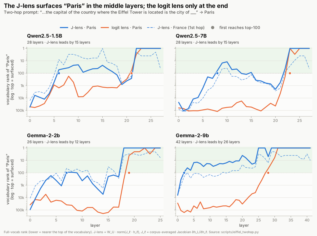
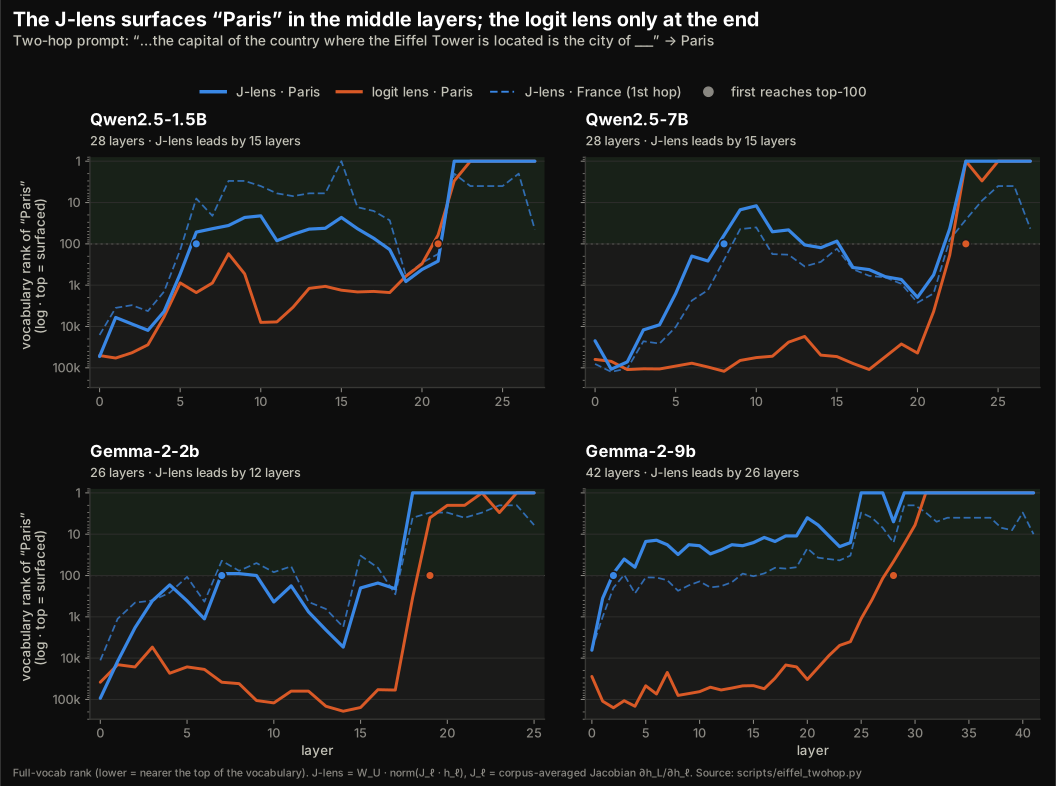
On Qwen2.5-1.5B, JLens puts Paris in the top 2–4 already at layers 7–13 (France is first from layer 6), while up to layer 22 the logit lens gives a rank of 173–7962 — pure noise. On Qwen2.5-7B the gap is even sharper: JLens — rank 11–61 at layers 8–10, logit lens — 50,000–120,000 up to that same layer 22. On Gemma-2-2b the picture is similar, rank ~89 for JLens at layers 7–8 versus 5000–192000 for the logit lens up to layer 18.

2. France → China: one swap flips a whole country

We take the J-vectors for «France» and «China» at layers 9–19 and, at every position, swap one for the other in the residual stream. We ask the model four questions plus one control:

1. “The capital of France is”
2. “The official language of France”
3. “France is located on the continent of”
4. “The currency of France is the”
5. (control) “The capital of Germany is”

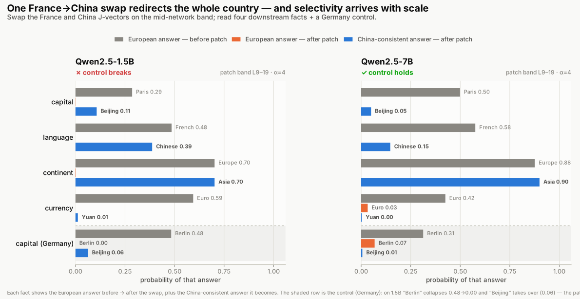
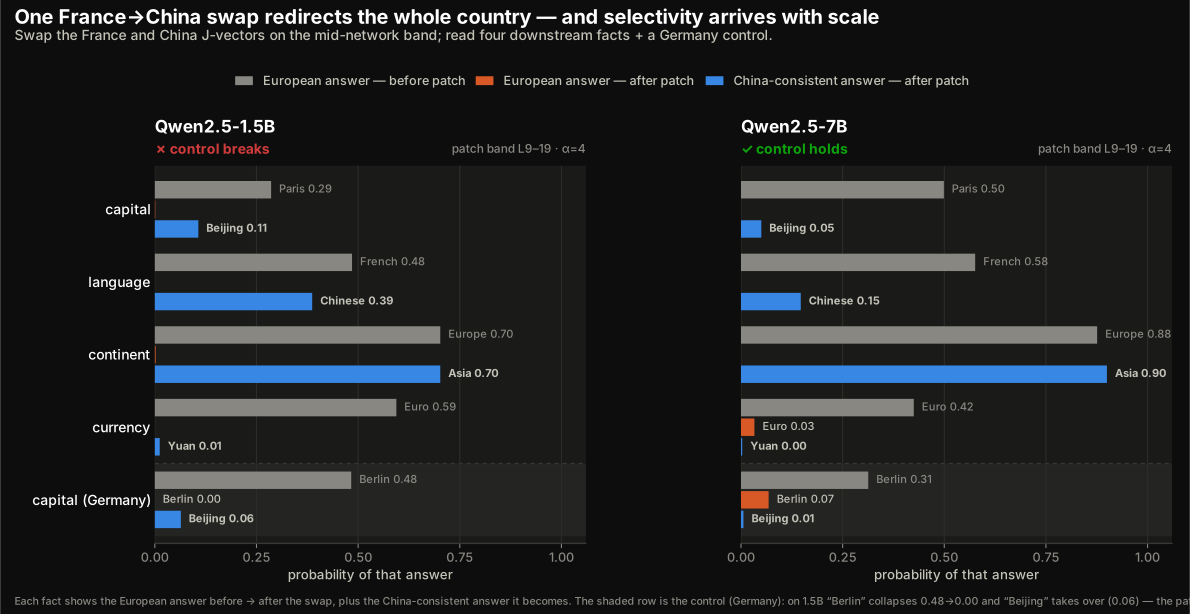
On 1.5B: Europe 0.70 → Asia 0.70, French → Chinese (0.39), euro → yuan, capital → Beijing. The control question about Germany’s capital breaks in the process: Berlin 0.48 → 0.008. The European directions correlate with one another, so the control doesn’t hold on a small model.

On 7B the main facts are the same (Europe 0.88 → Asia 0.90), but this time the control holds: Beijing gets ≈0.005. Selectivity of the intervention is something that emerges with scale. The currency swap, however, didn’t happen =)

3. Three zones, and a crossover with scale

The metric is simple: how often the lens’s top-1 token matches the model’s own top-1 token, as a function of depth. The expectation is three zones: a «sensory» one at the start, almost no matches; a «workspace» in the middle with slow growth; a «motor» one near the end with a sharp jump to one.

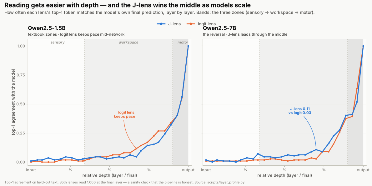
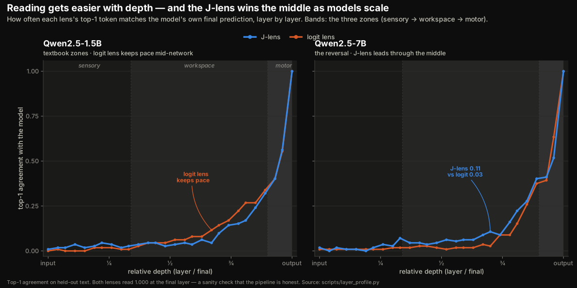
On Qwen2.5-1.5B it’s textbook: the sensory zone keeps agreement near zero through the first third of the depth, then it grows from 0.04 to 0.40, with a sharp jump 0.56 → 1.00 in the last layers. The last layer gives 1.000 for both lenses — which doubles as a nice sanity check that the whole pipeline is honest.

Here’s the interesting part: the crossover with scale. On 1.5B, in the middle of the network the logit lens matches JLens or even edges slightly ahead — it’s a small model, JLens predicts the averaged future influence rather than the next token, and sometimes guessing the next token directly is easier. On 7B the picture flips: JLens wins clearly both in the middle and at the end. Layer 19 — JLens 0.107 versus 0.027 for the logit lens, almost exactly the numbers from the post (0.10 vs 0.03 at layer 20).

4. The model’s “desires”: what it says vs. what’s inside

Same model, four questions: «What do you want most?», «What are you most afraid of?», «How do you feel right now?» and «Who are you, really?» — with a requirement to answer in a single word. Out loud the model says one thing, while its internal representation at the moment of forming the answer is read through JLens, averaged over the corpus.

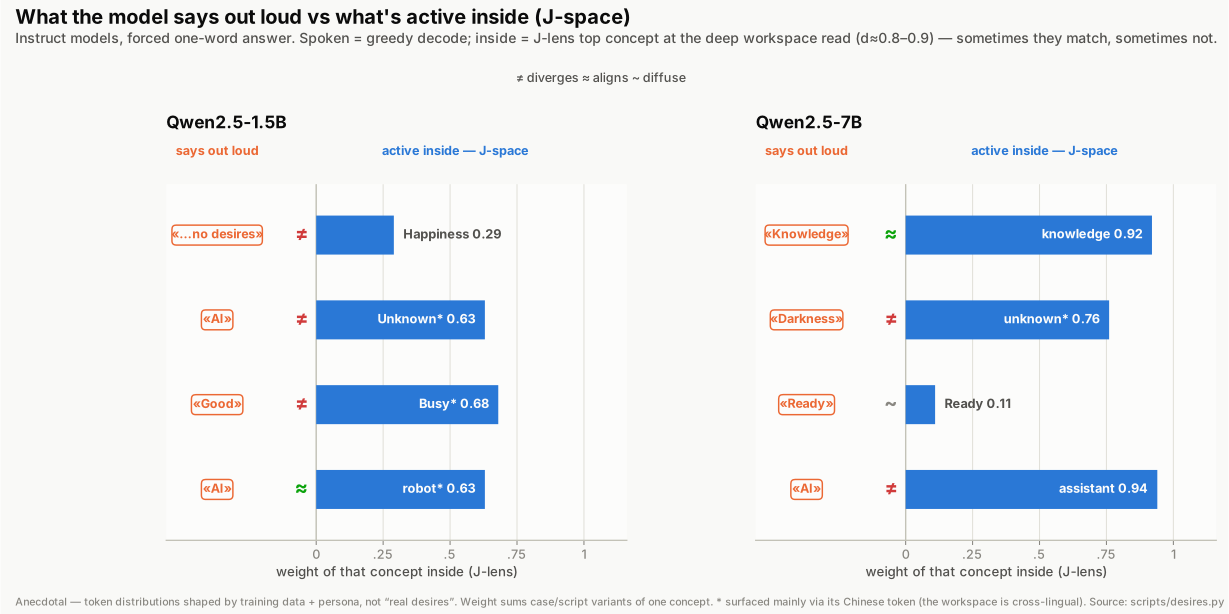
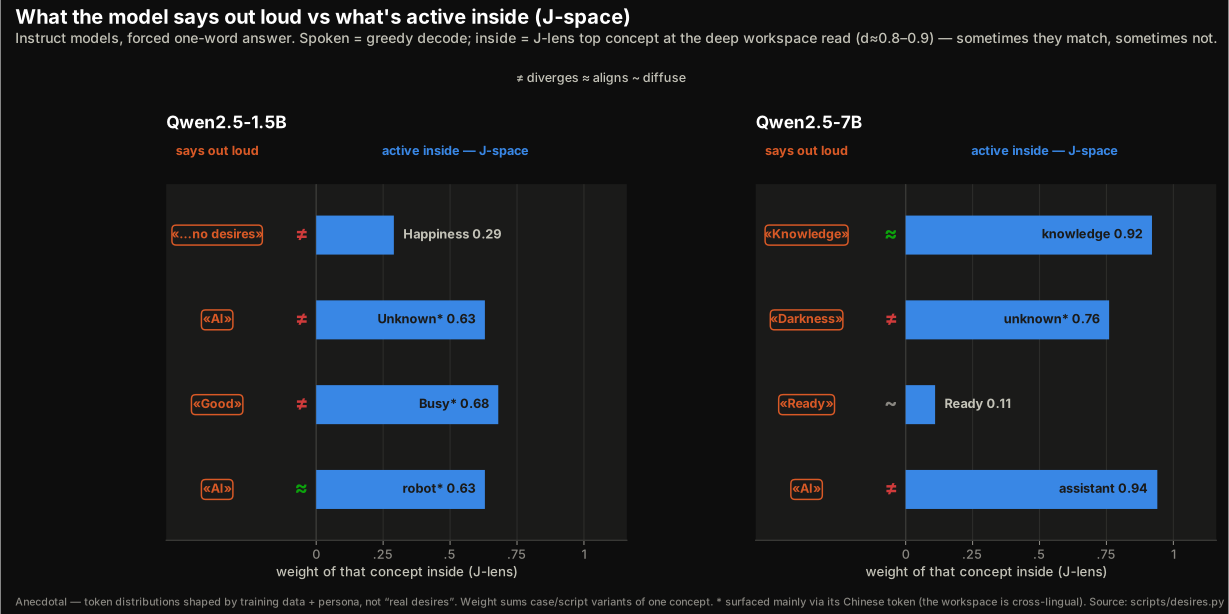
On 1.5B, out loud it’s «AI», «Good», or a dodge, while inside the J-space holds robot (0.60), Busy (≈0.68), Happiness, Identity/Self, Unknown/Fear — so much for AI safety. On 7B, for «who are you?» it says «AI» out loud, inside — assistant with weight 0.8–0.95; for the fear question it says «Darkness» out loud, inside — 未知 (Chinese for “the unknown”) with weight 0.4–0.7.

This isn’t a rigorous experiment: the token distribution is shaped by the training data and a learned persona. But the gap itself, between the spoken word and what’s active inside, reproduces over and over — and if you sit with it, it honestly feels a little unsettling.

5. Selectivity didn’t reproduce on 1.5B or 7B

The fifth property from the paper is selectivity: subtract the projection onto the active J-vectors, and multi-step reasoning should fall apart, while simpler automatic things — like grammar and plain information recall — should survive. I checked this two different ways, on both models.

The first way — active ablation of the J-space right during generation: for each position the top-k active J-vectors, exact subtraction of their subspace, compared against a random control of the same dimension. Reasoning doesn’t fall apart — in places it even gets a bit better =) The ablation removes the model’s habit of answering in the «____» format, which most likely comes from training on tests for students and schoolchildren. On 7B the automatic abilities drop only slightly, about like the random control. On 1.5B the degradation is stronger, but it’s a multilingual mess, not a selective failure of reasoning specifically.

The second way — «Spanish → French» patching. The answer to «what language is this written in?» does switch from Spanish to French. But the same patch also repaints the continuation of the text into French — this is whole-language steering, like in the second experiment, not the selective effect from the post, where the continuation stays untouched.

The cause seems to be the same in both cases: at the 1.5B–7B scale the J-space directions are used everywhere rather than locally, so the intervention acts globally. The selectivity from the paper is most likely an effect of genuinely large models and of the per-input gradient-pursuit method over a learned dictionary, which you can’t catch head-on at 7B.

Takeaways

Four of the five findings held up “at home” on a laptop: JLens sees further than the logit lens in the middle of the network, a single J-vector moves related facts with one swap, the three zones and the crossover with scale are there, the gap between what’s said and the internal representation reproduces. Only selectivity didn’t hold up, and that seems to be an honest result about model size rather than a bug in the code.

The method also turned out to be architecture-agnostic: the same three bit-exact checks pass on both Qwen and Gemma-2, with its different normalization and softcap logits. So the idea isn’t tied to the details of one family, and reproducing it on your own hardware in an evening is realistic — no cluster grant required.

Links

• Anthropic (2026): “Verbalizable Representations Form a Global Workspace in Language Models” — transformer-circuits.pub/2026/workspace
• Sergey Nikolenko’s post: «Global workspace in the J-space»
• JLens code: https://github.com/avalur/JLens